[Paper Review] Data for "Phase transition in Random Circuit Sampling"

A. Morvan, B. Villalonga+182 more|arXiv (Cornell University)|Apr 21, 2023

Neural Networks and Applications38 citations

TL;DR

The paper demonstrates experimentally and theoretically two phase transitions in Random Circuit Sampling (RCS) driven by circuit depth and per-cycle noise, using XEB to map transitions between a highly complex, hard-to-spoof regime and a weakly correlated regime; it also proves beyond-classical computation with 67 qubits at 32 cycles.

ABSTRACT

Purpose This dataset defines the Random Quantum Circuits (RQCs) used in our paper "Phase transition in Random Circuit Sampling" and lists the bitstrings observed in the experimental executions of the circuits on the Sycamore processor. See [1] for more details about the experiment. This data upload is modeled after that of [5]. Background Circuit parameters RQCs posted here are uniquely identifiedusing the following parameters: `n`: number of qubits (69, 70), `m`: number of cycles (04, 06, 08, ..., 28, 30), `s`: seed for the pseudo-random number generator (000, 001, ..., 595), `patches`: the number of patches, `p`: sequence of coupler activation patterns (`ABCD`, `ABCDCDAB`), `num_sq`: the number of distinct single-qubit gates (3, 8), the date on which the data was collected, included in yymmdd format in the filename, and `phase_match`: included in the file name if phase matching was performed. See Figure S25 in [2] and Figure 3 of [1] for the coupler activation patterns and Figure 4 of [1] for illustrations of the patches. Also see code snippets below for visualizing the patches and activation patterns from the provided circuits.When `num_sq` is 8, the single-qubit gates are chosen randomly from \(Z^p X^{1/2} Z^{-p}\), with \(p \in \{-1, -3/4, -1/2, -1/4, 0, 1/4, 1/2, 3/4 \}\), whereas when `num_sq` is 3, they are chosen randomly from among \(\sqrt X\), \(\sqrt Y\), and \(\sqrt W\). Phase matching is described in Appendix C.1 of [1]. Note that circuits which share the same seed `s` share the same initial gate sequence. Content description For each RQC there are four files in the dataset: * original RQC specification in QSIM format, named `circuit_\*.qsim`, * derived RQC specificaton as python code using cirq, named `circuit_\*.py`, * derived RQC specification in QASM format, named `circuit_\*.qasm`, * bitstrings observed in experiments, named `measurements_\*.txt`. The asterisk \* in the names above stands for a string specifying the parameters identifying a RQC. For example,`circuit_n70_m24_s00_patches3_pABCD_num_sq8_221014_phase_match.qasm` contains the definition of the 70-qubit, 24-cycle RQC with PRNG seed 0, 3 patches, a simplifiable sequence of coupler activation patterns (i.e. ABCD), and 8 distinct single-qubit gates, taken on October 14, 2022, with phase matching, in the QASM format. Files are grouped by parameters `n`, `m`, and `patches` and into compressed tarballs. For example, tarball `n69_m04_patches2.tar.gz` contains all RQCs and measurement files for circuits with 69 qubits, 4 cycles, and 2 patches. Circuit file formats QSIM format First line specifies the number of qubits n. Each subsequent line specifies a single gate and consists of moment number, gate name and one or two qubits as a number in 0..n-1 optionally followed by gate parameters. The circuits use the following gates: * `x_1_2`: parameter-free, single-qubit pi/2 rotation around the X axis of the Bloch sphere, see equation (45) in section VII of [2], * `y_1_2`: parameter-free, single-qubit pi/2 rotation around the Y axis of the Bloch sphere, see equation (46) in section VII of [2], * `hz_1_2`: parameter-free, single-qubit pi/2 rotation around the X+Y axis of the Bloch sphere, see equation (47) in section VII of [2], * `rz`: single-qubit rotation around the Z axis of the Bloch sphere through the angle specified in radians by the gate's sole parameter, * `fsim`: two-qubit gate corresponding to the composition of the iSWAP and CPHASE gates and taking two parameters in radians: theta (the negative iSWAP angle) and phi (the CPHASE angle), see equation (48) in section VII of [2]. Note that the two-qubit gates executed in our experiments on Sycamore belong to the five-parameter family of two-qubit gates that preserve the number of 0 and 1 states of the qubits. Each such gate can be decomposed into one fsim gate and four rz gates. Therefore, one cycle consisting of one application ofsingle-qubit gates and one application of two-qubit gates is represented in the file using four moments. The first moment contains `x_1_2`, `y_1_2` and `hz_1_2` gates. The other three moments use `rz` and `fsim` gates to describe the two-qubit gates used in the experiments. See section VII in [2] for more details about the Sycamore gates and their decomposition. Qubits are specified as numbers in 0..n-1 and hence do not directly indicate qubit location on the device. Python/cirq format Each python file defines two variables: QUBIT_ORDER and CIRCUIT. The former is a python list object containing `cirq.GridQubit` objects initialized with therow and column of each qubit on the device. The latter is a `cirq.Circuit` object initialized with all gate operations contained in the circuit. The files have been tested using cirq version 1.2.0.dev20230613162638. The following code snippet illustrates how one can use cirq and our circuit definitions to compute output state amplitudes: $ python -i circuit_n70_m24_s00_patches3_pABCD_num_sq8_221014_phase_match.py >>> cirq.final_wavefunction(CIRCUIT, qubit_order=QUBIT_ORDER) array([ 0.00263724+0.00337646j, 0.0009332 +0.00111853j, -0.0007809 +0.00386362j, ..., 0.00574739-0.00027827j, -0.00254766+0.00299345j, 0.00396056+0.00312335j], dtype=complex64) See [3] for more details about cirq. QASM format Each QASM file has been generated using cirq and specifies the RQC decomposed into CNOT and single-qubit gates. The files have been generated using cirq. See [4] for more details about the format. Measurements file format Each line contains the bitstring obtained in a single execution of the RQC on Sycamore. The first, left-most position corresponds to the qubit 0 in QSIM format and the first qubit in the `QUBIT_ORDER` list in the python/cirq files. To visualize the patches After loading `CIRCUIT` from the appropriate `.py` file, the following code snippet can be used to visualize the patches: import cirq import matplotlib.pyplot as plt pairs = set() for moment in CIRCUIT: for op in moment.operations: q = op.qubits if len(q) > 1: assert len(q) == 2 pairs.add(tuple(sorted(q))) d = {p:1 for p in pairs} heatmap = cirq.TwoQubitInteractionHeatmap(d) _, ax = plt.subplots(figsize=(8, 8)) _ = heatmap.plot(ax) Visualize the activation patterns The activation pattern sequence can also be visualized in a similar manner. After loading `CIRCUIT` from the appropriate `.py` pyle, the following code snippet can be used to visualize the activation patterns: import cirq import matplotlib.pyplot as plt def has_two_qubit_gates(moment): has = False for op in moment.operations: if len(op.qubits) > 1: has = True break return has def plot_pairs(moment): pairs = set() for op in moment.operations: q = op.qubits if len(q) > 1: assert len(q) == 2 pairs.add( tuple(sorted(q)) ) d = {p:1 for p in pairs} heatmap = cirq.TwoQubitInteractionHeatmap(d) _, ax = plt.subplots(figsize=(8, 8)) _ = heatmap.plot(ax) return ax moments = [_ for _ in CIRCUIT if has_two_qubit_gates(_)] moment_to_visualize = moments[0] # iterate through this manually plot_pairs(moment_to_visualize) Content listing The dataset includes the following tarball files: n69_m04_patches2.tar.gz (80 files) n69_m04_patches3.tar.gz (80 files) n69_m06_patches2.tar.gz (80 files) n69_m06_patches3.tar.gz (80 files) n69_m08_patches2.tar.gz (80 files) n69_m08_patches3.tar.gz (80 files) n69_m10_patches2.tar.gz (80 files) n69_m10_patches3.tar.gz (80 files) n69_m12_patches2.tar.gz (80 files) n69_m12_patches3.tar.gz (80 files) n69_m14_patches2.tar.gz (80 files) n69_m14_patches3.tar.gz (80 files) n69_m16_patches2.tar.gz (80 files) n69_m16_patches3.tar.gz (80 files) n69_m18_patches2.tar.gz (80 files) n69_m18_patches3.tar.gz (80 files) n69_m20_patches2.tar.gz (80 files) n69_m20_patches3.tar.gz (80 files) n69_m22_patches2.tar.gz (80 files) n69_m22_patches3.tar.gz (80 files) n69_m24_patches1.tar.gz (4 files) n69_m24_patches2.tar.gz (80 files) n69_m24_patches3.tar.gz (80 files) n69_m26_patches2.tar.gz (80 files) n69_m26_patches3.tar.gz (80 files) n69_m28_patches2.tar.gz (80 files) n69_m28_patches3.tar.gz (80 files) n69_m30_patches2.tar.gz (80 files) n69_m30_patches3.tar.gz (80 files) n70_m16_patches2.tar.gz (960 files) n70_m16_patches3.tar.gz (1040 files) n70_m16_patches9.tar.gz (160 files) n70_m18_patches2.tar.gz (960 files) n70_m18_patches3.tar.gz (1040 files) n70_m18_patches9.tar.gz (160 files) n70_m20_patches2.tar.gz (960 files) n70_m20_patches3.tar.gz (1040 files) n70_m20_patches9.tar.gz (160 files) n70_m22_patches2.tar.gz (960 files) n70_m22_patches3.tar.gz (1040 files) n70_m22_patches9.tar.gz (160 files) n70_m24_patches1.tar.gz (56 files) n70_m24_patches2.tar.gz (960 files) n70_m24_patches3.tar.gz (1040 files) n70_m24_patches9.tar.gz (160 files) n70_m26_patches1.tar.gz (4 files) n70_m26_patches2.tar.gz (880 files) n70_m26_patches3.tar.gz (960 files) n70_m26_patches9.tar.gz (160 files) Additionally, the file Figures 2 and 3 data.zip contains processed data (9 files in Pickle format) that are shown in Figures 2 and 3 of the paper. References [1] Google AI Quantum and collaborators, "Phase transition in Random Circuit Sampling". arXiv:2304.11119 [2] Google AI Quantum and collaborators, Supplementary information for “Quantum supremacy using a programmable superconducting processor”. arXiv:1910.11333 [3] Cirq: A Python framework for creating, editing, and invoking Noisy Intermediate Scale Quantum (NISQ) circuits, https://github.com/quantumlib/Cirq. [4] Cross, Andrew W.; Bishop, Lev S.; Smolin, John A.; Gambetta, Jay M. "Open Quantum Assembly Language", arXiv:1707.03429 [5] Martinis, John M. et al. (2022), "Quantum supremacy using a programmable superconducting processor", Dryad, Dataset, https://doi.org/10.5061/dryad.k6t1rj8

Motivation & Objective

• Motivate how noise and circuit depth limit the usable Hilbert space in near-term quantum processors.
• Show experimentally that two distinct phase transitions govern RCS behavior under XEB.
• Develop a weak-link model to analytically and experimentally identify noise-driven transitions.
• Demonstrate a beyond-classical RCS experiment on a 67-qubit device.
• Quantify the computational hardness versus fidelity and discuss classical simulation feasibility.

Proposed method

• Use linear cross-entropy benchmarking (XEB) to quantify fidelity and phase behavior as a function of circuit depth (cycles) and system size.
• Implement 1D and 2D superconducting qubit layouts with Haar random single-qubit gates and iSWAP-like entanglers.
• Introduce a weak-link model to separate subsystems and study noise versus entanglement dynamics.
• Define and analyze an order parameter F^d / XEB to identify noise-induced phase transitions.
• Carry out a 67-qubit, 32-cycle RCS experiment and verify fidelity via Loschmidt echo and patch-based XEB validation.
• Compare experimental results with numerical simulations, tensor-network contractions, and matrix-product-state analyses.

Figure 1: Phase transitions in Random Circuit Sampling: One phase transition goes between a concentrated output distribution of bitstrings from RCS at low number of cycles to a broad or anti-concentrated distribution. There is a second phase transition in a noisy system. Strong enough error per cycl

Experimental results

Research questions

• RQ1 What are the phase transitions in RCS as a function of circuit depth and per-cycle noise?
• RQ2 Can XEB reliably diagnose the boundary between a globally entangled, computationally complex phase and a noise-dominated regime?
• RQ3 How does a weak-link coupling affect the transition between subsystems under noise?
• RQ4 Is a 67-qubit RCS circuit at 32 cycles beyond classical simulation capabilities under realistic noise?
• RQ5 How do 1D vs 2D circuit architectures influence the location and nature of these transitions?

Key findings

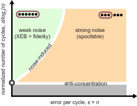
• There exist two phase transitions observable with XEB: a dynamical transition with circuit depth and a noise-driven quantum phase transition controlled by error per cycle.
• XEB transitions indicate a regime where correlations span the full system (weak noise) versus a regime where subsystems are effectively uncorrelated (strong noise).
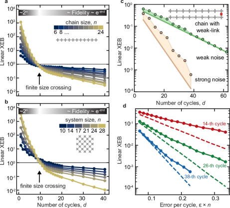
• A weak-link model captures the noise-driven transition and predicts a boundary where XEB no longer faithfully reflects fidelity; experiments show crossover behavior consistent with the model.
• In 1D and 2D layouts, a crossing point in XEB curves occurs at specific cycle numbers, indicating the dynamical phase transition; higher cycle counts lead to anti-concentration and then fidelity-dominated XEB.
• A 67-qubit Sycamore experiment at 32 cycles achieves fidelity and hardness consistent with beyond-classical performance, with classical simulation costs estimated to be prohibitively large under realistic memory constraints.
• Numerical and experimental results collectively bound the critical noise rate εn and show 2D patterns yield robust weak-noise regimes across system sizes.

Figure 2: Phase transitions in the Linear Cross-entropy: At low number of cycles, XEB grows with the size of the system. In a noiseless device, XEB will converge to 1 with the number of cycles. In the presence of noise XEB becomes an estimator of the system fidelity. In a and b , we observe experime