[论文解读] Parameter identifiability, parameter estimation and model prediction for differential equation models

Matthew J. Simpson, Ruth E. Baker|arXiv (Cornell University)|May 13, 2024

Fault Detection and Control Systems被引用 6

一句话总结

本文提出基于似然的方法，用于评估 ODE、PDE 和 BVP 模型中参数的可识别性、估计参数以及将预测中的不确定性传播到预测中，并在 GitHub 上提供开源的 Julia 代码。

ABSTRACT

Interpreting data with mathematical models is an important aspect of real-world industrial and applied mathematical modeling. Often we are interested to understand the extent to which a particular set of data informs and constrains model parameters. This question is closely related to the concept of parameter identifiability, and in this article we present a series of computational exercises to introduce tools that can be used to assess parameter identifiability, estimate parameters and generate model predictions. Taking a likelihood-based approach, we show that very similar ideas and algorithms can be used to deal with a range of different mathematical modeling frameworks. The exercises and results presented in this article are supported by a suite of open access codes that can be accessed on GitHub.

研究动机与目标

• 引入一个基于似然的框架，以评估数据在微分方程模型中对模型参数的约束程度。
• 展示对 ODE、PDE 和 BVP 问题使用轮廓似然进行参数估计和可识别性分析。
• 展示参数不确定性如何通过预测区间转化为预测的不确定性。
• 强调噪声模型的问题以及在实现可识别性时可能需要重新参数化。

提出的方法

• 使用一个似然框架，其中观测数据被建模为模型解的带噪声的评估（高斯或对数正态噪声）。
• 将对数似然视为对数据点的求和，将参数值与模型解 T(t) 或 u(x,t) 联系起来。
• 通过数值优化（Nelder–Mead via NLopt）估计最大似然参数。
• 构建归一化对数似然和单变量轮廓似然，以评估可识别性并基于卡方阈值计算近似的 95% 置信区间。
• 从置信集抽样以将参数不确定性传播到预测，生成预测区间。
• 将这些步骤应用于：(i) ODE 牛顿冷却定律、(ii) PDE 对流-扩散模型，以及 (iii) 稳态 BVP 的形态发生物质梯度，包括在可识别性受损时的重新参数化。

Figure 1: Left panel: synthetic data (blue dots) showing observations $T^{\textrm{o}}(t)$ at $t=0,10,20,\ldots,100$ superimposed with the MLE solution (solid red) with $\hat{\theta}=(\hat{T_{a}},\hat{k})^{\mathsf{T}}=(25.386,0.053)^{\mathsf{T}}$ . Right panel: heat map of $\bar{\ell}(\theta\mid T^{\

实验结果

研究问题

• RQ1 在给定特定数据集时，ODE、PDE 与 BVP 模型的参数有多大程度的可识别性？
• RQ2 参数的最大似然估计是什么，对它们的置信度有多大？
• RQ3 参数不确定性如何传播到模型预测的不确定性？
• RQ4 在直接参数不可识别时，重新参数化是否能恢复可识别性？

主要发现

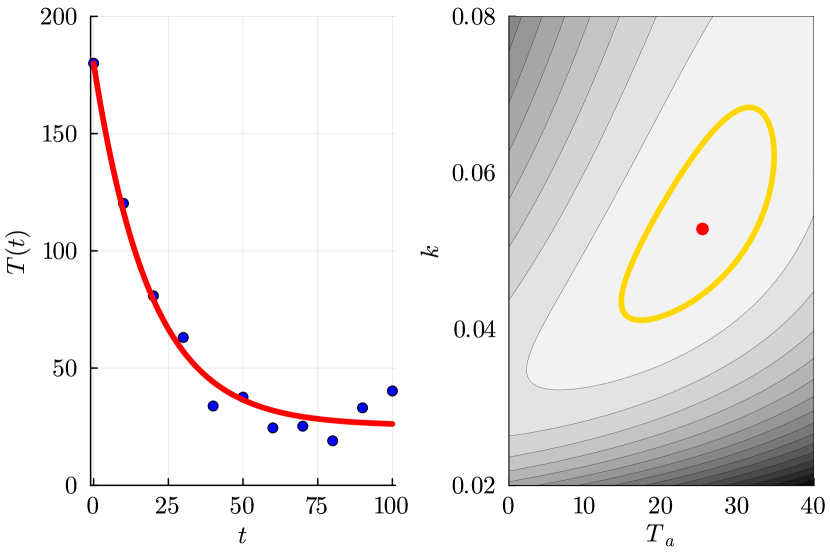
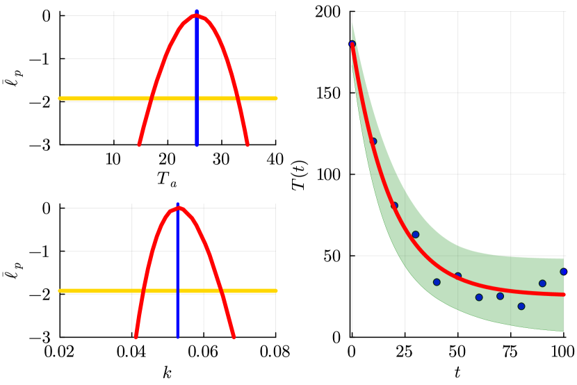
• 对于 ODE 冷却模型，MLE 为 θ̂ = (Tâ, k̂) = (25.386, 0.053)，95% 置信区间为 Ta ∈ [16.977, 32.983]，k ∈ [0.0432, 0.0648]。
• Ta 和 k 的单变量轮廓似然在 ODE 示例中显示单峰可识别性。
• 对于具有四个参数 (u0, h, D, v) 的 PDE 对流-扩散模型，所有参数在轮廓似然下均具有实际可识别性，且有明显峰值和 95% 置信区间：u0 ∈ [0.839, 1.156]，h ∈ [42.939, 58.043]，D ∈ [6.227, 13.686]，v ∈ [0.990, 1.060]。
• 对 PDE 使用乘法中性对数正态噪声模型导致预测区间非负，并且相比加性高斯噪声具有更好的一致性。
• 在一个简单的 BVP 示例中，参数 (J, D, k) 因结构依赖于 J/√(kD) 和 √(k/D) 而不可识别；重新参数化为 (α, β)，其中 α = J/√(kD) 且 β = √(k/D)，得到可识别的量 α 和 β 及其各自的轮廓似然。
• 本文表明在原始参数化不可识别时，重新参数化可以恢复可识别性，并且可以构建反映组合参数与噪声不确定性的预测区间。
• 在各个示例中，该方法同时给出点估计和不确定性量化，且 GitHub 上提供了开源的 Julia 代码以便复现。

Figure 2: Left panel: Univariate profile likelihood functions for $T_{a}$ and $k$ , as indicated (solid red). Each profile indicates the MLE (solid blue) and the $95\%$ threshold $\bar{\ell}^{*}=-\Delta_{0.95,1}/2\approx-1.921$ contour (solid gold). The 95% confidence intervals are $T_{a}\in[16.977,