[论文解读] Data for "Phase transition in Random Circuit Sampling"

A. Morvan, B. Villalonga+182 more|arXiv (Cornell University)|Apr 21, 2023

Neural Networks and Applications被引用 38

一句话总结

本文通过实验和理论展示在 Random Circuit Sampling (RCS) 中由电路深度和每周期噪声驱动的两种相变，使用 XEB 将过渡映射到高度复杂、难以伪造的状态与弱相关性状态之间；并且证明在 67 比特、32 轮次下超越经典计算能力。

ABSTRACT

Purpose This dataset defines the Random Quantum Circuits (RQCs) used in our paper "Phase transition in Random Circuit Sampling" and lists the bitstrings observed in the experimental executions of the circuits on the Sycamore processor. See [1] for more details about the experiment. This data upload is modeled after that of [5]. Background Circuit parameters RQCs posted here are uniquely identifiedusing the following parameters: `n`: number of qubits (69, 70), `m`: number of cycles (04, 06, 08, ..., 28, 30), `s`: seed for the pseudo-random number generator (000, 001, ..., 595), `patches`: the number of patches, `p`: sequence of coupler activation patterns (`ABCD`, `ABCDCDAB`), `num_sq`: the number of distinct single-qubit gates (3, 8), the date on which the data was collected, included in yymmdd format in the filename, and `phase_match`: included in the file name if phase matching was performed. See Figure S25 in [2] and Figure 3 of [1] for the coupler activation patterns and Figure 4 of [1] for illustrations of the patches. Also see code snippets below for visualizing the patches and activation patterns from the provided circuits.When `num_sq` is 8, the single-qubit gates are chosen randomly from \(Z^p X^{1/2} Z^{-p}\), with \(p \in \{-1, -3/4, -1/2, -1/4, 0, 1/4, 1/2, 3/4 \}\), whereas when `num_sq` is 3, they are chosen randomly from among \(\sqrt X\), \(\sqrt Y\), and \(\sqrt W\). Phase matching is described in Appendix C.1 of [1]. Note that circuits which share the same seed `s` share the same initial gate sequence. Content description For each RQC there are four files in the dataset: * original RQC specification in QSIM format, named `circuit_\*.qsim`, * derived RQC specificaton as python code using cirq, named `circuit_\*.py`, * derived RQC specification in QASM format, named `circuit_\*.qasm`, * bitstrings observed in experiments, named `measurements_\*.txt`. The asterisk \* in the names above stands for a string specifying the parameters identifying a RQC. For example,`circuit_n70_m24_s00_patches3_pABCD_num_sq8_221014_phase_match.qasm` contains the definition of the 70-qubit, 24-cycle RQC with PRNG seed 0, 3 patches, a simplifiable sequence of coupler activation patterns (i.e. ABCD), and 8 distinct single-qubit gates, taken on October 14, 2022, with phase matching, in the QASM format. Files are grouped by parameters `n`, `m`, and `patches` and into compressed tarballs. For example, tarball `n69_m04_patches2.tar.gz` contains all RQCs and measurement files for circuits with 69 qubits, 4 cycles, and 2 patches. Circuit file formats QSIM format First line specifies the number of qubits n. Each subsequent line specifies a single gate and consists of moment number, gate name and one or two qubits as a number in 0..n-1 optionally followed by gate parameters. The circuits use the following gates: * `x_1_2`: parameter-free, single-qubit pi/2 rotation around the X axis of the Bloch sphere, see equation (45) in section VII of [2], * `y_1_2`: parameter-free, single-qubit pi/2 rotation around the Y axis of the Bloch sphere, see equation (46) in section VII of [2], * `hz_1_2`: parameter-free, single-qubit pi/2 rotation around the X+Y axis of the Bloch sphere, see equation (47) in section VII of [2], * `rz`: single-qubit rotation around the Z axis of the Bloch sphere through the angle specified in radians by the gate's sole parameter, * `fsim`: two-qubit gate corresponding to the composition of the iSWAP and CPHASE gates and taking two parameters in radians: theta (the negative iSWAP angle) and phi (the CPHASE angle), see equation (48) in section VII of [2]. Note that the two-qubit gates executed in our experiments on Sycamore belong to the five-parameter family of two-qubit gates that preserve the number of 0 and 1 states of the qubits. Each such gate can be decomposed into one fsim gate and four rz gates. Therefore, one cycle consisting of one application ofsingle-qubit gates and one application of two-qubit gates is represented in the file using four moments. The first moment contains `x_1_2`, `y_1_2` and `hz_1_2` gates. The other three moments use `rz` and `fsim` gates to describe the two-qubit gates used in the experiments. See section VII in [2] for more details about the Sycamore gates and their decomposition. Qubits are specified as numbers in 0..n-1 and hence do not directly indicate qubit location on the device. Python/cirq format Each python file defines two variables: QUBIT_ORDER and CIRCUIT. The former is a python list object containing `cirq.GridQubit` objects initialized with therow and column of each qubit on the device. The latter is a `cirq.Circuit` object initialized with all gate operations contained in the circuit. The files have been tested using cirq version 1.2.0.dev20230613162638. The following code snippet illustrates how one can use cirq and our circuit definitions to compute output state amplitudes: $ python -i circuit_n70_m24_s00_patches3_pABCD_num_sq8_221014_phase_match.py >>> cirq.final_wavefunction(CIRCUIT, qubit_order=QUBIT_ORDER) array([ 0.00263724+0.00337646j, 0.0009332 +0.00111853j, -0.0007809 +0.00386362j, ..., 0.00574739-0.00027827j, -0.00254766+0.00299345j, 0.00396056+0.00312335j], dtype=complex64) See [3] for more details about cirq. QASM format Each QASM file has been generated using cirq and specifies the RQC decomposed into CNOT and single-qubit gates. The files have been generated using cirq. See [4] for more details about the format. Measurements file format Each line contains the bitstring obtained in a single execution of the RQC on Sycamore. The first, left-most position corresponds to the qubit 0 in QSIM format and the first qubit in the `QUBIT_ORDER` list in the python/cirq files. To visualize the patches After loading `CIRCUIT` from the appropriate `.py` file, the following code snippet can be used to visualize the patches: import cirq import matplotlib.pyplot as plt pairs = set() for moment in CIRCUIT: for op in moment.operations: q = op.qubits if len(q) > 1: assert len(q) == 2 pairs.add(tuple(sorted(q))) d = {p:1 for p in pairs} heatmap = cirq.TwoQubitInteractionHeatmap(d) _, ax = plt.subplots(figsize=(8, 8)) _ = heatmap.plot(ax) Visualize the activation patterns The activation pattern sequence can also be visualized in a similar manner. After loading `CIRCUIT` from the appropriate `.py` pyle, the following code snippet can be used to visualize the activation patterns: import cirq import matplotlib.pyplot as plt def has_two_qubit_gates(moment): has = False for op in moment.operations: if len(op.qubits) > 1: has = True break return has def plot_pairs(moment): pairs = set() for op in moment.operations: q = op.qubits if len(q) > 1: assert len(q) == 2 pairs.add( tuple(sorted(q)) ) d = {p:1 for p in pairs} heatmap = cirq.TwoQubitInteractionHeatmap(d) _, ax = plt.subplots(figsize=(8, 8)) _ = heatmap.plot(ax) return ax moments = [_ for _ in CIRCUIT if has_two_qubit_gates(_)] moment_to_visualize = moments[0] # iterate through this manually plot_pairs(moment_to_visualize) Content listing The dataset includes the following tarball files: n69_m04_patches2.tar.gz (80 files) n69_m04_patches3.tar.gz (80 files) n69_m06_patches2.tar.gz (80 files) n69_m06_patches3.tar.gz (80 files) n69_m08_patches2.tar.gz (80 files) n69_m08_patches3.tar.gz (80 files) n69_m10_patches2.tar.gz (80 files) n69_m10_patches3.tar.gz (80 files) n69_m12_patches2.tar.gz (80 files) n69_m12_patches3.tar.gz (80 files) n69_m14_patches2.tar.gz (80 files) n69_m14_patches3.tar.gz (80 files) n69_m16_patches2.tar.gz (80 files) n69_m16_patches3.tar.gz (80 files) n69_m18_patches2.tar.gz (80 files) n69_m18_patches3.tar.gz (80 files) n69_m20_patches2.tar.gz (80 files) n69_m20_patches3.tar.gz (80 files) n69_m22_patches2.tar.gz (80 files) n69_m22_patches3.tar.gz (80 files) n69_m24_patches1.tar.gz (4 files) n69_m24_patches2.tar.gz (80 files) n69_m24_patches3.tar.gz (80 files) n69_m26_patches2.tar.gz (80 files) n69_m26_patches3.tar.gz (80 files) n69_m28_patches2.tar.gz (80 files) n69_m28_patches3.tar.gz (80 files) n69_m30_patches2.tar.gz (80 files) n69_m30_patches3.tar.gz (80 files) n70_m16_patches2.tar.gz (960 files) n70_m16_patches3.tar.gz (1040 files) n70_m16_patches9.tar.gz (160 files) n70_m18_patches2.tar.gz (960 files) n70_m18_patches3.tar.gz (1040 files) n70_m18_patches9.tar.gz (160 files) n70_m20_patches2.tar.gz (960 files) n70_m20_patches3.tar.gz (1040 files) n70_m20_patches9.tar.gz (160 files) n70_m22_patches2.tar.gz (960 files) n70_m22_patches3.tar.gz (1040 files) n70_m22_patches9.tar.gz (160 files) n70_m24_patches1.tar.gz (56 files) n70_m24_patches2.tar.gz (960 files) n70_m24_patches3.tar.gz (1040 files) n70_m24_patches9.tar.gz (160 files) n70_m26_patches1.tar.gz (4 files) n70_m26_patches2.tar.gz (880 files) n70_m26_patches3.tar.gz (960 files) n70_m26_patches9.tar.gz (160 files) Additionally, the file Figures 2 and 3 data.zip contains processed data (9 files in Pickle format) that are shown in Figures 2 and 3 of the paper. References [1] Google AI Quantum and collaborators, "Phase transition in Random Circuit Sampling". arXiv:2304.11119 [2] Google AI Quantum and collaborators, Supplementary information for “Quantum supremacy using a programmable superconducting processor”. arXiv:1910.11333 [3] Cirq: A Python framework for creating, editing, and invoking Noisy Intermediate Scale Quantum (NISQ) circuits, https://github.com/quantumlib/Cirq. [4] Cross, Andrew W.; Bishop, Lev S.; Smolin, John A.; Gambetta, Jay M. "Open Quantum Assembly Language", arXiv:1707.03429 [5] Martinis, John M. et al. (2022), "Quantum supremacy using a programmable superconducting processor", Dryad, Dataset, https://doi.org/10.5061/dryad.k6t1rj8

研究动机与目标

• 激发/说明噪声和电路深度如何限制近端量子处理器可用的希尔伯特空间。
• 实验证实在 XEB 下有两种不同的相变支配 RCS 行为。
• 建立一个弱连结模型，以解析地和实验地识别噪声驱动的相变。
• 在 67-qubit 设备上演示超越经典的 RCS 实验。
• 量化计算难度与保真度之间的关系，并讨论经典仿真的可行性。

提出的方法

• 使用线性交叉熵基准测试（XEB）来量化保真度和相行为，随着电路深度（周期）和系统规模变化。
• 实现包含 Haar 随机单量子比特门和 iSWAP 类纠缠门的 1D 与 2D 超导量子比特布局。
• 引入弱连结模型以分离子系统并研究噪声与纠缠动力学。
• 定义并分析序参量 F^d / XEB 以识别噪声诱导的相变。
• 进行 67-qubit、32 循环的 RCS 实验，并通过 Loschmidt 回声和基于补丁的 XEB 验证来验证保真度。
• 将实验结果与数值仿真、张量网络收缩及矩阵乘积态分析进行比较。

Figure 1: Phase transitions in Random Circuit Sampling: One phase transition goes between a concentrated output distribution of bitstrings from RCS at low number of cycles to a broad or anti-concentrated distribution. There is a second phase transition in a noisy system. Strong enough error per cycl

实验结果

研究问题

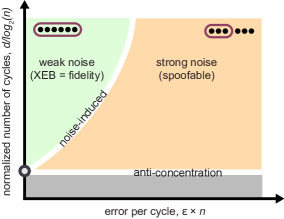
• RQ1 RCS 随着电路深度和每周期噪声的函数有哪些相变？
• RQ2 XEB 能否可靠地诊断全局纠缠、计算复杂性相与噪声主导的状态之间的边界？
• RQ3 弱连结耦合在噪声下如何影响子系统之间的转变？
• RQ4 在现实噪声下，67-qubit、32 循环的 RCS 电路是否超越经典仿真能力？
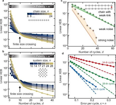
• RQ5 1D 与 2D 电路结构如何影响这些相变的位置及性质？

主要发现

• 存在两种可通过 XEB 观测的相变：一种随电路深度的动力学相变，另一种由每周期误差控制的噪声驱动量子相变。
• XEB 转变指示一个相关性遍及整个系统的状态（弱噪声）与一个子系统实质上不相关的状态（强噪声）之间的区间。
• 弱连结模型捕捉噪声驱动的转变，并预测一个边界，在该边界上 XEB 不再如实地反映保真度；实验显示出与模型一致的拐点行为。
• 在 1D 和 2D 布局中，XEB 曲线在特定循环数出现交叉点，指示动力学相变；更高的循环数导致反集中化，然后是保真度主导的 XEB。
• 67-qubit Sycamore 实验在 32 循环下达到的保真度和难度与超越经典性能一致，在现实内存约束下，经典仿真的成本被估计为非常高。
• 数值与实验结果共同限定了临界噪声率 εn，并显示 2D 模式在不同系统规模下产生稳健的弱噪声区。

Figure 2: Phase transitions in the Linear Cross-entropy: At low number of cycles, XEB grows with the size of the system. In a noiseless device, XEB will converge to 1 with the number of cycles. In the presence of noise XEB becomes an estimator of the system fidelity. In a and b , we observe experime