[论文解读] Efficient Neural Network Approaches for Conditional Optimal Transport with Applications in Bayesian Inference

Zheyu Oliver Wang, Ricardo Baptista+3 more|arXiv (Cornell University)|Oct 25, 2023

Gaussian Processes and Bayesian Inference被引用 5

一句话总结

本文提出了两种基于深度学习的方法——PCP-Map 和 COT-Flow——用于在贝叶斯推断中高效求解条件最优传输（COT）问题。通过使用神经网络参数化单调传输映射（部分凸网络与正则化归一化流），这些方法实现了从复杂条件后验分布中快速采样与密度估计，在高维反问题中相比最先进方法在收敛速度与数值精度方面表现更优。

ABSTRACT

We present two neural network approaches that approximate the solutions of static and dynamic $\unicode{x1D450}\unicode{x1D45C}\unicode{x1D45B}\unicode{x1D451}\unicode{x1D456}\unicode{x1D461}\unicode{x1D456}\unicode{x1D45C}\unicode{x1D45B}\unicode{x1D44E}\unicode{x1D459}\unicode{x0020}\unicode{x1D45C}\unicode{x1D45D}\unicode{x1D461}\unicode{x1D456}\unicode{x1D45A}\unicode{x1D44E}\unicode{x1D459}\unicode{x0020}\unicode{x1D461}\unicode{x1D45F}\unicode{x1D44E}\unicode{x1D45B}\unicode{x1D460}\unicode{x1D45D}\unicode{x1D45C}\unicode{x1D45F}\unicode{x1D461}$ (COT) problems. Both approaches enable conditional sampling and conditional density estimation, which are core tasks in Bayesian inference$\unicode{x2013}$particularly in the simulation-based ($\unicode{x201C}$likelihood-free$\unicode{x201D}$) setting. Our methods represent the target conditional distribution as a transformation of a tractable reference distribution. Obtaining such a transformation, chosen here to be an approximation of the COT map, is computationally challenging even in moderate dimensions. To improve scalability, our numerical algorithms use neural networks to parameterize candidate maps and further exploit the structure of the COT problem. Our static approach approximates the map as the gradient of a partially input-convex neural network. It uses a novel numerical implementation to increase computational efficiency compared to state-of-the-art alternatives. Our dynamic approach approximates the conditional optimal transport via the flow map of a regularized neural ODE; compared to the static approach, it is slower to train but offers more modeling choices and can lead to faster sampling. We demonstrate both algorithms numerically, comparing them with competing state-of-the-art approaches, using benchmark datasets and simulation-based Bayesian inverse problems.

研究动机与目标

• 解决高维贝叶斯推断中条件最优传输（COT）问题的计算不可行性。
• 开发可扩展、可微分的神经网络参数化方法，用于 COT 映射，以实现快速采样与密度估计。
• 通过最大似然训练替代对抗性训练，克服度量传输中对抗训练的局限性。
• 实现跨多个条件变量的摊销条件采样，降低每次推断的计算成本。
• 为似然或先验不可计算时的条件后验近似提供实用且可复现的框架。

提出的方法

• PCP-Map 将条件传输映射参数化为部分输入凸神经网络（PICNN）的梯度，通过凸势函数确保单调性与唯一性。
• COT-Flow 通过正则化神经 ODE 的流动建模条件传输，利用神经网络参数化的速度场强制保守动力学。
• 两种方法均通过观测目标样本的最大似然进行训练，避免对抗优化，支持端到端反向传播。
• PCP-Map 方法使用凸优化进行采样，而 COT-Flow 使用 ODE 积分，训练完成后采样速度更快。
• 采用两步超参数搜索启发式方法，以在多种数据集与问题设置中识别鲁棒的配置。
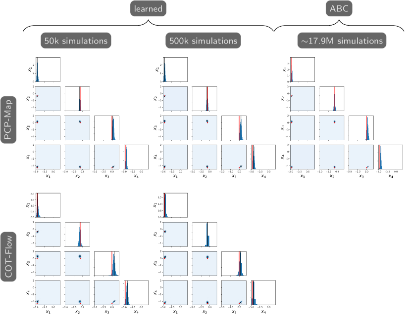
• 方法应用于基准反问题，包括随机 Lotka-Volterra 方程与一维浅水方程，条件维度较高。

Figure 2: Posterior samples in log scale and MAP point quality comparisons between proposed approaches and ABC with ${\bf x}^{*}=(0.01,0.5,1,0.01)^{\top}$ . Left : posterior samples generated by proposed approaches trained on 50k samples. Middle : posterior samples generated by proposed approaches t

实验结果

研究问题

• RQ1 神经网络能否在保持单调性与唯一性等理想理论性质的同时，高效参数化条件最优传输映射？
• RQ2 在贝叶斯推断中，基于最大似然的传输映射训练与对抗训练相比，在收敛速度与样本质量方面表现如何？
• RQ3 在不同 COT 建模形式中，特别是静态（PCP-Map）与动态（COT-Flow）方法之间，训练时间与采样速度之间的权衡如何？
• RQ4 当传统基于网格或多项式逼近的方法失效时，这些方法在高维问题中的可扩展性如何？
• RQ5 这些方法对超参数选择的鲁棒性如何？简单的启发式方法是否能提升在多样化应用场景中的配置选择效率？

主要发现

• 在包含 14 个有效参数与 3,500 个观测值的高维反问题中，PCP-Map 的收敛时间约为 715 秒。
• 尽管 PCP-Map 为静态建模，其收敛速度仍快于摊销的 CP-Flow 方法。
• COT-Flow 因采用 ODE 积分，采样速度优于 PCP-Map，尤其在速度场充分训练后优势更明显。
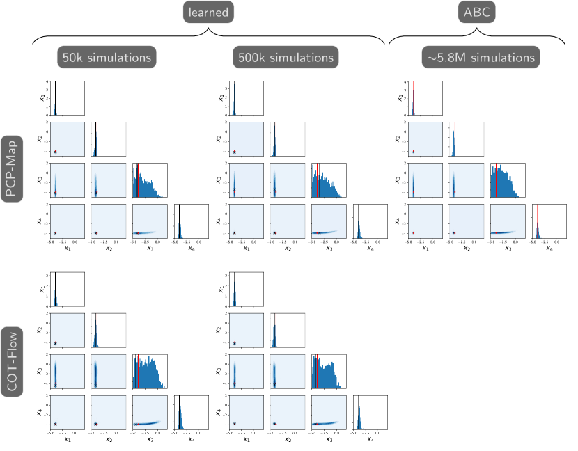
• 在 1D 浅水方程问题中，两种方法在数值精度上均优于 SMC-ABC，尽管 ABC 具有强大的理论保证。
• PCP-Map 在广泛超参数范围内（特征宽度、上下文宽度、深度）表现出一致性能，仅需三个关键超参数。
• 在似然或先验计算不可行的设置中，方法依然有效，证明其在涉及 SDE 或遗留代码的真实世界反问题中的实用性。

Figure 3: Posterior samples log scale and MAP point quality comparisons between proposed approaches and ABC with ${\bf x}^{*}=(0.02,0.02,0.02,0.02)^{\top}$ . Left : posterior samples generated by proposed approaches trained on 50k samples. Middle : posterior samples generated by proposed approaches