[论文解读] Low depth algorithms for quantum amplitude estimation

Tudor Giurgică-Tiron, Iordanis Kerenidis+3 more|arXiv (Cornell University)|Dec 6, 2020

Quantum Computing Algorithms and Architecture被引用 5

一句话总结

本文提出了两种低深度的量子振幅估计算法——幂律振幅估计（Power Law AE）与QoPrime AE——在电路深度与量子预言机调用次数之间实现了最优权衡。通过在经典与标准量子标度之间插值，这些算法使近场含噪声中等规模量子（NISQ）设备上的蒙特卡洛方法实现实际的量子加速，其中幂律振幅估计在噪声环境下表现出更优的实验性能。

ABSTRACT

We design and analyze two new low depth algorithms for amplitude estimation (AE) achieving an optimal tradeoff between the quantum speedup and circuit depth. For $β\in (0,1]$, our algorithms require $N= ilde{O}( \frac{1}{ ε^{1+β}})$ oracle calls and require the oracle to be called sequentially $D= O( \frac{1}{ ε^{1-β}})$ times to perform amplitude estimation within additive error $ε$. These algorithms interpolate between the classical algorithm $(β=1)$ and the standard quantum algorithm ($β=0$) and achieve a tradeoff $ND= O(1/ε^{2})$. These algorithms bring quantum speedups for Monte Carlo methods closer to realization, as they can provide speedups with shallower circuits. The first algorithm (Power law AE) uses power law schedules in the framework introduced by Suzuki et al \cite{S20}. The algorithm works for $β\in (0,1]$ and has provable correctness guarantees when the log-likelihood function satisfies regularity conditions required for the Bernstein Von-Mises theorem. The second algorithm (QoPrime AE) uses the Chinese remainder theorem for combining lower depth estimates to achieve higher accuracy. The algorithm works for discrete $β=q/k$ where $k \geq 2$ is the number of distinct coprime moduli used by the algorithm and $1 \leq q \leq k-1$, and has a fully rigorous correctness proof. We analyze both algorithms in the presence of depolarizing noise and provide numerical comparisons with the state of the art amplitude estimation algorithms.

研究动机与目标

• 解决标准量子振幅估计中电路深度过高的问题，该问题限制了其在近场含噪声中等规模量子（NISQ）设备上的适用性。
• 设计能够降低电路深度同时保持振幅估计量子加速的算法，尤其适用于蒙特卡洛方法与机器学习应用。
• 实现预言机调用次数与电路深度之间的权衡，插值于经典（$\beta=1$）与标准量子（$\beta=0$）标度之间。
• 在现实噪声条件（尤其是比特消相干噪声）下提供严格的正确性保证，以确保在当前硬件上的实际可行性。
• 与最先进的算法（如IQAE）进行基准测试，证明其在抗噪声能力与资源开销方面具有优势。

提出的方法

• 提出幂律振幅估计（Power Law AE），在Suzuki等人框架中使用幂律调度，预言机调用次数与深度分别满足$N = \tilde{O}(\epsilon^{-(1+\beta)})$与$D = O(\epsilon^{-(1-\beta)})$，其中$\beta \in (0,1]$。
• 提出QoPrime AE，通过中国剩余定理将多个低深度振幅估计结合使用互质模数，实现更高精度的同时降低深度。
• 通过完全严格的证明确保QoPrime AE的理论正确性，适用于离散$\beta = q/k$情形，其中$k \geq 2$且$1 \leq q \leq k-1$。
• 在分析中使用切尔诺夫不等式与精确二项分布置信区间，以高精度限制失败概率并估计预言机调用次数。
• 通过设定噪声下限$\gamma$来建模比特消相干噪声，确保深度不超过$O(\gamma^{-1})$，以避免置信区间指数衰减。
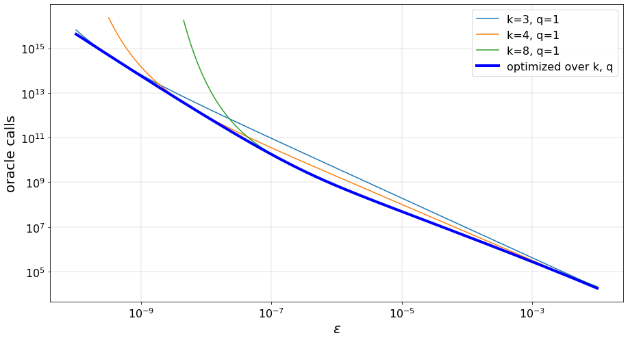
• 利用理论边界与实验模拟联合优化算法参数（如$\beta$、$k$、$q$），在噪声条件下最小化预言机调用次数与深度。

Figure 1: Convergence of the coprime finding routine. The algorithm finds $k$ adjacent coprimes $n_{1}$ , $n_{2}$ , …, $n_{k}$ such that their product $N=n_{1}\dots n_{k}$ is close to $\pi/\epsilon$ . Both the smallest coprime $n_{1}$ (approaching 1 from below) and the largest coprime $n_{k}$ (appro

实验结果

研究问题

• RQ1 能否在显著降低电路深度的同时，仍为实际NISQ设备保留量子加速的振幅估计？
• RQ2 振幅估计中预言机调用次数与电路深度之间的最优权衡是什么？是否能通过连续参数$\beta$进行参数化？
• RQ3 在现实的比特消相干噪声下，所提算法表现如何？是否避免了IQAE等高深度算法中常见的指数级开销？
• RQ4 中国剩余定理能否有效应用于量子振幅估计，以将多个低深度估计组合为高精度结果？
• RQ5 理论边界对预言机调用次数与深度的估计，在噪声模拟中与实际性能的匹配程度如何？

主要发现

• 幂律振幅估计（Power Law AE）实现了$N = \tilde{O}(\epsilon^{-(1+\beta)})$次预言机调用与$D = O(\epsilon^{-(1-\beta)})$的电路深度，其中$\beta \in (0,1]$，在经典（$\beta=1$）与标准量子（$\beta=0$）标度之间实现插值。
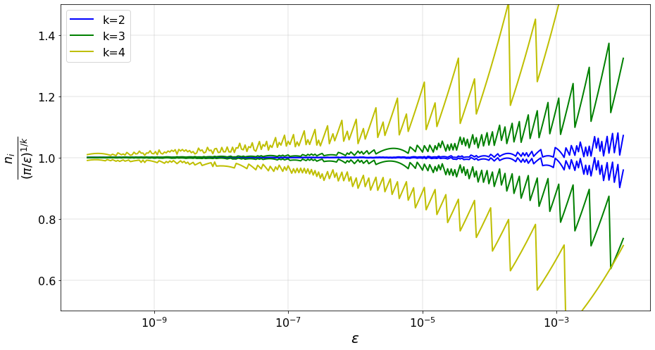
• QoPrime AE在离散$\beta = q/k$情形下提供了完全严格的正确性证明，实验性能显示在广泛$\epsilon$与噪声率范围内，常数前因子$C < 10$。
• 在比特消相干噪声率$\gamma$下，两种算法在$\epsilon \ll \gamma$时平滑过渡至经典标度，避免了IQAE中常见的预言机调用指数级膨胀。
• 数值模拟表明，幂律振幅估计在实际中优于IQAE，尤其在噪声环境下，因其能平滑过渡至经典性能而无指数级开销。
• QoPrime AE的最大预言机深度受$O(\gamma^{-1})$限制，防止在精度受噪声限制时深度过度增长，从而避免样本需求指数级上升。
• QoPrime AE的预言机调用次数理论上限较为保守；实验结果表明其性能更优，原因在于实际计算中使用了精确二项分布置信区间，而非理论分析中的切尔诺夫近似。

Figure 2: The behavior of the oracle call dependency in ( 22 ) for several values of parameters $k$ and $q$ , and for fixed noise level $\gamma=10^{-5}$ and probability of failure $\delta=10^{-5}$ . When taking the minimum over the family of curves parametrized by all valid $k$ and $q$ (here assumed