[论文解读] Physics-informed neural networks with residual/gradient-based adaptive sampling methods for solving PDEs with sharp solutions

Zhiping Mao, Xuhui Meng|arXiv (Cornell University)|Feb 16, 2023

Model Reduction and Neural Networks被引用 5

一句话总结

本文提出一种结合残差与梯度的自适应采样方法（ASMs）的物理信息神经网络（PINNs），以提升求解具有尖锐解的偏微分方程（PDEs）时的精度。通过在残差或解梯度较大的区域迭代添加残差点，ASM II（同时使用两种指标）在收敛性、稳定性和精度方面均优于标准PINNs及仅基于残差的ASM I。

ABSTRACT

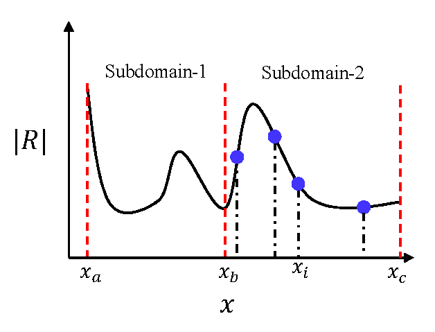
We consider solving the forward and inverse PDEs which have sharp solutions using physics-informed neural networks (PINNs) in this work. In particular, to better capture the sharpness of the solution, we propose adaptive sampling methods (ASMs) based on the residual and the gradient of the solution. We first present a residual only based ASM algorithm denoted by ASM I. In this approach, we first train the neural network by using a small number of residual points and divide the computational domain into a certain number of sub-domains, we then add new residual points in the sub-domain which has the largest mean absolute value of the residual, and those points which have largest absolute values of the residual in this sub-domain will be added as new residual points. We further develop a second type of ASM algorithm (denoted by ASM II) based on both the residual and the gradient of the solution due to the fact that only the residual may be not able to efficiently capture the sharpness of the solution. The procedure of ASM II is almost the same as that of ASM I except that in ASM II, we add new residual points which not only have large residual but also large gradient. To demonstrate the effectiveness of the present methods, we employ both ASM I and ASM II to solve a number of PDEs, including Burger equation, compressible Euler equation, Poisson equation over an L-shape domain as well as high-dimensional Poisson equation. It has been shown from the numerical results that the sharp solutions can be well approximated by using either ASM I or ASM II algorithm, and both methods deliver much more accurate solution than original PINNs with the same number of residual points. Moreover, the ASM II algorithm has better performance in terms of accuracy, efficiency and stability compared with the ASM I algorithm.

研究动机与目标

• 解决使用物理信息神经网络（PINNs）求解具有尖锐解的偏微分方程（PDEs）时面临的挑战，此类方法常因收敛性差和精度低而表现不佳。
• 克服均匀采样或基于先验知识的残差采样方法的局限性，提出基于动态细化高误差区域或陡峭梯度区域的自适应采样策略。
• 提升复杂几何结构与高维问题中正问题与逆问题的解精度与训练稳定性。
• 当尖锐特征靠近边界时，将自适应细化扩展至边界条件，以增强整体解的保真度。
• 展示结合残差与梯度信息可实现更鲁棒、更高效的PINNs采样策略。

提出的方法

• 提出ASM I：一种自适应采样方法，其在平均绝对残差最大的子域中添加新残差点，并选择残差值最大的点。
• 开发ASM II：一种增强型方法，结合残差与梯度幅值，向残差大且解梯度大的区域添加点，以更准确捕捉尖锐特征。
• 采用域分解方法将计算域划分为S个子域，以实现局部误差与梯度评估。
• 应用高斯求积法计算子域内积分残差与梯度范数，用于自适应细化决策。
• 通过在解幅值较大的边界点处添加边界点，实现自适应边界采样，当尖锐特征靠近边界时尤为有效。
• 在每次迭代中使用Adam与L-BFGS优化器迭代训练PINN，并应用自适应细化，直至收敛或达到最大迭代次数。

Figure 1: Schematic of PINNs. Yellow dots: inputs of the NN, blue dots: activation function, green dots $\tilde{u}$ : output of the neural network (which is used to approximate the solution of the PDE), orange dots: differential operator, $R$ represents the residual of the PDE, $Loss_{Data}$ represe

实验结果

研究问题

• RQ1 与均匀采样或仅基于残差的采样相比，基于残差与梯度的自适应采样是否能提升PINNs在求解具有尖锐解的PDEs时的精度？
• RQ2 在PINNs中引入解梯度信息如何提升自适应采样过程的稳定性与效率？
• RQ3 当尖锐特征位于域边界时，边界附近的自适应采样在多大程度上提升了解的精度？
• RQ4 在不同PDE（包括非线性与高维问题）中，所提出的ASMs（ASM I与ASM II）在收敛速度、精度与鲁棒性方面表现如何？
• RQ5 与标准PINN方法相比，所提出的自适应采样策略是否能显著减少达到高精度所需的残差点数量？

主要发现

• 在高维Poisson方程（$d=9$）上，ASM II（结合残差与梯度信息）的收敛速度更快，且$ L^∞ $误差显著低于ASM I与标准PINNs。
• 在L形域Poisson问题中，采用自适应边界采样的方法相比基线PINN与仅基于残差的自适应采样，显著提升了精度、稳定性和效率。
• 在可压缩Euler方程与Burgers方程上，ASM I与ASM II在相同残差点数量下均优于标准PINNs，且ASM II展现出更优的精度与稳定性。
• ASM II中引入梯度信息可更有效地检测与细化不连续性与尖锐层，从而实现更优的解分辨率。
• 在高维问题中，ASM II以更少的残差点实现了比ASM I更高的精度，证明了其更优的采样效率。
• 基于残差与梯度双重信息的自适应细化策略可带来更稳定的训练过程，尤其在具有复杂或局部尖锐特征的问题中表现更优。

Figure 2: Schematic for the computation of mean value of the absolute value ( $\mathcal{E}$ ) in a sub-domain. Based on the Gaussian quadrature, the $\mathcal{E}$ is calculated as $\mathcal{E}=\frac{1}{x_{c}-x_{b}}\int^{x_{c}}_{x_{b}}|R(x)|dx\approx\frac{1}{x_{c}-x_{b}}\sum^{N}_{i}\omega_{i}|R(x_{i}