[논문 리뷰] Data for "Phase transition in Random Circuit Sampling"

A. Morvan, B. Villalonga외 182명|arXiv (Cornell University)|2023. 04. 21.

Neural Networks and Applications인용 수 38

한 줄 요약

본 논문은 Random Circuit Sampling (RCS)의 두 가지 위상 전이를 회로 깊이와 사이클당 잡음에 의해 실험적으로 및 이론적으로 입증하고, XEB를 사용해 매우 복잡하고 위조하기 어려운(regime)와 약하게 상관된(regime) 사이의 전이를 매핑한다; 또한 32 사이클에서 67 큐비트로 초-고전 계산을 증명한다.

ABSTRACT

Purpose This dataset defines the Random Quantum Circuits (RQCs) used in our paper "Phase transition in Random Circuit Sampling" and lists the bitstrings observed in the experimental executions of the circuits on the Sycamore processor. See [1] for more details about the experiment. This data upload is modeled after that of [5]. Background Circuit parameters RQCs posted here are uniquely identifiedusing the following parameters: `n`: number of qubits (69, 70), `m`: number of cycles (04, 06, 08, ..., 28, 30), `s`: seed for the pseudo-random number generator (000, 001, ..., 595), `patches`: the number of patches, `p`: sequence of coupler activation patterns (`ABCD`, `ABCDCDAB`), `num_sq`: the number of distinct single-qubit gates (3, 8), the date on which the data was collected, included in yymmdd format in the filename, and `phase_match`: included in the file name if phase matching was performed. See Figure S25 in [2] and Figure 3 of [1] for the coupler activation patterns and Figure 4 of [1] for illustrations of the patches. Also see code snippets below for visualizing the patches and activation patterns from the provided circuits.When `num_sq` is 8, the single-qubit gates are chosen randomly from \(Z^p X^{1/2} Z^{-p}\), with \(p \in \{-1, -3/4, -1/2, -1/4, 0, 1/4, 1/2, 3/4 \}\), whereas when `num_sq` is 3, they are chosen randomly from among \(\sqrt X\), \(\sqrt Y\), and \(\sqrt W\). Phase matching is described in Appendix C.1 of [1]. Note that circuits which share the same seed `s` share the same initial gate sequence. Content description For each RQC there are four files in the dataset: * original RQC specification in QSIM format, named `circuit_\*.qsim`, * derived RQC specificaton as python code using cirq, named `circuit_\*.py`, * derived RQC specification in QASM format, named `circuit_\*.qasm`, * bitstrings observed in experiments, named `measurements_\*.txt`. The asterisk \* in the names above stands for a string specifying the parameters identifying a RQC. For example,`circuit_n70_m24_s00_patches3_pABCD_num_sq8_221014_phase_match.qasm` contains the definition of the 70-qubit, 24-cycle RQC with PRNG seed 0, 3 patches, a simplifiable sequence of coupler activation patterns (i.e. ABCD), and 8 distinct single-qubit gates, taken on October 14, 2022, with phase matching, in the QASM format. Files are grouped by parameters `n`, `m`, and `patches` and into compressed tarballs. For example, tarball `n69_m04_patches2.tar.gz` contains all RQCs and measurement files for circuits with 69 qubits, 4 cycles, and 2 patches. Circuit file formats QSIM format First line specifies the number of qubits n. Each subsequent line specifies a single gate and consists of moment number, gate name and one or two qubits as a number in 0..n-1 optionally followed by gate parameters. The circuits use the following gates: * `x_1_2`: parameter-free, single-qubit pi/2 rotation around the X axis of the Bloch sphere, see equation (45) in section VII of [2], * `y_1_2`: parameter-free, single-qubit pi/2 rotation around the Y axis of the Bloch sphere, see equation (46) in section VII of [2], * `hz_1_2`: parameter-free, single-qubit pi/2 rotation around the X+Y axis of the Bloch sphere, see equation (47) in section VII of [2], * `rz`: single-qubit rotation around the Z axis of the Bloch sphere through the angle specified in radians by the gate's sole parameter, * `fsim`: two-qubit gate corresponding to the composition of the iSWAP and CPHASE gates and taking two parameters in radians: theta (the negative iSWAP angle) and phi (the CPHASE angle), see equation (48) in section VII of [2]. Note that the two-qubit gates executed in our experiments on Sycamore belong to the five-parameter family of two-qubit gates that preserve the number of 0 and 1 states of the qubits. Each such gate can be decomposed into one fsim gate and four rz gates. Therefore, one cycle consisting of one application ofsingle-qubit gates and one application of two-qubit gates is represented in the file using four moments. The first moment contains `x_1_2`, `y_1_2` and `hz_1_2` gates. The other three moments use `rz` and `fsim` gates to describe the two-qubit gates used in the experiments. See section VII in [2] for more details about the Sycamore gates and their decomposition. Qubits are specified as numbers in 0..n-1 and hence do not directly indicate qubit location on the device. Python/cirq format Each python file defines two variables: QUBIT_ORDER and CIRCUIT. The former is a python list object containing `cirq.GridQubit` objects initialized with therow and column of each qubit on the device. The latter is a `cirq.Circuit` object initialized with all gate operations contained in the circuit. The files have been tested using cirq version 1.2.0.dev20230613162638. The following code snippet illustrates how one can use cirq and our circuit definitions to compute output state amplitudes: $ python -i circuit_n70_m24_s00_patches3_pABCD_num_sq8_221014_phase_match.py >>> cirq.final_wavefunction(CIRCUIT, qubit_order=QUBIT_ORDER) array([ 0.00263724+0.00337646j, 0.0009332 +0.00111853j, -0.0007809 +0.00386362j, ..., 0.00574739-0.00027827j, -0.00254766+0.00299345j, 0.00396056+0.00312335j], dtype=complex64) See [3] for more details about cirq. QASM format Each QASM file has been generated using cirq and specifies the RQC decomposed into CNOT and single-qubit gates. The files have been generated using cirq. See [4] for more details about the format. Measurements file format Each line contains the bitstring obtained in a single execution of the RQC on Sycamore. The first, left-most position corresponds to the qubit 0 in QSIM format and the first qubit in the `QUBIT_ORDER` list in the python/cirq files. To visualize the patches After loading `CIRCUIT` from the appropriate `.py` file, the following code snippet can be used to visualize the patches: import cirq import matplotlib.pyplot as plt pairs = set() for moment in CIRCUIT: for op in moment.operations: q = op.qubits if len(q) > 1: assert len(q) == 2 pairs.add(tuple(sorted(q))) d = {p:1 for p in pairs} heatmap = cirq.TwoQubitInteractionHeatmap(d) _, ax = plt.subplots(figsize=(8, 8)) _ = heatmap.plot(ax) Visualize the activation patterns The activation pattern sequence can also be visualized in a similar manner. After loading `CIRCUIT` from the appropriate `.py` pyle, the following code snippet can be used to visualize the activation patterns: import cirq import matplotlib.pyplot as plt def has_two_qubit_gates(moment): has = False for op in moment.operations: if len(op.qubits) > 1: has = True break return has def plot_pairs(moment): pairs = set() for op in moment.operations: q = op.qubits if len(q) > 1: assert len(q) == 2 pairs.add( tuple(sorted(q)) ) d = {p:1 for p in pairs} heatmap = cirq.TwoQubitInteractionHeatmap(d) _, ax = plt.subplots(figsize=(8, 8)) _ = heatmap.plot(ax) return ax moments = [_ for _ in CIRCUIT if has_two_qubit_gates(_)] moment_to_visualize = moments[0] # iterate through this manually plot_pairs(moment_to_visualize) Content listing The dataset includes the following tarball files: n69_m04_patches2.tar.gz (80 files) n69_m04_patches3.tar.gz (80 files) n69_m06_patches2.tar.gz (80 files) n69_m06_patches3.tar.gz (80 files) n69_m08_patches2.tar.gz (80 files) n69_m08_patches3.tar.gz (80 files) n69_m10_patches2.tar.gz (80 files) n69_m10_patches3.tar.gz (80 files) n69_m12_patches2.tar.gz (80 files) n69_m12_patches3.tar.gz (80 files) n69_m14_patches2.tar.gz (80 files) n69_m14_patches3.tar.gz (80 files) n69_m16_patches2.tar.gz (80 files) n69_m16_patches3.tar.gz (80 files) n69_m18_patches2.tar.gz (80 files) n69_m18_patches3.tar.gz (80 files) n69_m20_patches2.tar.gz (80 files) n69_m20_patches3.tar.gz (80 files) n69_m22_patches2.tar.gz (80 files) n69_m22_patches3.tar.gz (80 files) n69_m24_patches1.tar.gz (4 files) n69_m24_patches2.tar.gz (80 files) n69_m24_patches3.tar.gz (80 files) n69_m26_patches2.tar.gz (80 files) n69_m26_patches3.tar.gz (80 files) n69_m28_patches2.tar.gz (80 files) n69_m28_patches3.tar.gz (80 files) n69_m30_patches2.tar.gz (80 files) n69_m30_patches3.tar.gz (80 files) n70_m16_patches2.tar.gz (960 files) n70_m16_patches3.tar.gz (1040 files) n70_m16_patches9.tar.gz (160 files) n70_m18_patches2.tar.gz (960 files) n70_m18_patches3.tar.gz (1040 files) n70_m18_patches9.tar.gz (160 files) n70_m20_patches2.tar.gz (960 files) n70_m20_patches3.tar.gz (1040 files) n70_m20_patches9.tar.gz (160 files) n70_m22_patches2.tar.gz (960 files) n70_m22_patches3.tar.gz (1040 files) n70_m22_patches9.tar.gz (160 files) n70_m24_patches1.tar.gz (56 files) n70_m24_patches2.tar.gz (960 files) n70_m24_patches3.tar.gz (1040 files) n70_m24_patches9.tar.gz (160 files) n70_m26_patches1.tar.gz (4 files) n70_m26_patches2.tar.gz (880 files) n70_m26_patches3.tar.gz (960 files) n70_m26_patches9.tar.gz (160 files) Additionally, the file Figures 2 and 3 data.zip contains processed data (9 files in Pickle format) that are shown in Figures 2 and 3 of the paper. References [1] Google AI Quantum and collaborators, "Phase transition in Random Circuit Sampling". arXiv:2304.11119 [2] Google AI Quantum and collaborators, Supplementary information for “Quantum supremacy using a programmable superconducting processor”. arXiv:1910.11333 [3] Cirq: A Python framework for creating, editing, and invoking Noisy Intermediate Scale Quantum (NISQ) circuits, https://github.com/quantumlib/Cirq. [4] Cross, Andrew W.; Bishop, Lev S.; Smolin, John A.; Gambetta, Jay M. "Open Quantum Assembly Language", arXiv:1707.03429 [5] Martinis, John M. et al. (2022), "Quantum supremacy using a programmable superconducting processor", Dryad, Dataset, https://doi.org/10.5061/dryad.k6t1rj8

연구 동기 및 목표

• 노이즈와 회로 깊이가 근접형 양자 프로세서에서 사용 가능한 힐베르트 공간을 어떻게 제한하는지 동기를 부여한다.
• XEB 하에서 RCS 동작을 지배하는 두 가지 서로 다른 위상 전이를 실험적으로 보인다.
• 노이즈 주도 전이를 해석적으로이고 실험적으로 식별하기 위한 약한 연결 모델(weak-link model)을 개발한다.
• 67-큐비트 장치에서 초-고전(beyond-classical) RCS 실험을 시연한다.
• 충실도와 계산 난이도 사이의 관계를 계량하고 고전 시뮬레이션 가능성에 대해 논의한다.

제안 방법

• 회로 깊이(사이클) 및 시스템 크기에 따른 충실도와 위상 거동을 정량화하기 위해 선형 교차 엔트로피 벤치마킹 (XEB)을 사용한다.
• Haar 난수 단일 큐비트 게이트와 iSWAP 유사 얽힘기를 사용하여 1D 및 2D 초전도 큐비트 배치를 구현한다.
• 약한 연결 모델(weak-link model)을 도입하여 서브시스템을 분리하고 노이즈 대 얽힘 역학을 연구한다.
• 노이즈 유도 위상 전이를 식별하기 위해 차수계수 F^d / XEB를 정의하고 분석한다.
• 67-큐비트, 32-사이클 RCS 실험을 수행하고 Loschmidt 에코 및 패치 기반 XEB 검증으로 충실도를 확인한다.
• 실험 결과를 수치 시뮬레이션, 텐서-네트워크 수축, 및 행렬곱 상태 분석과 비교한다.

Figure 1: Phase transitions in Random Circuit Sampling: One phase transition goes between a concentrated output distribution of bitstrings from RCS at low number of cycles to a broad or anti-concentrated distribution. There is a second phase transition in a noisy system. Strong enough error per cycl

실험 결과

연구 질문

• RQ1 회로 깊이와 사이클당 노이즈의 함수로서 RCS의 위상 전이는 무엇인가?
• RQ2 XEB가 전역적으로 얽히고 계산적으로 복잡한 위상과 노이즈 지배된 영역 사이의 경계를 신뢰성 있게 진단할 수 있는가?
• RQ3 약한 연결 결합이 노이즈 하에서 서브시스템 간 전이에 어떤 영향을 미치는가?
• RQ4 현실적인 노이즈 하에서 32사이클의 67-큐비트 RCS 회로가 고전 시뮬레이션 능력의 경계를 넘는가?
• RQ5 1D 대 2D 회로 아키텍처가 이러한 전이의 위치와 특성에 어떻게 영향을 미치는가?

주요 결과

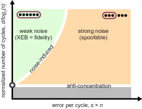
• XEB로 관찰 가능한 두 가지 위상 전이가 존재한다: 회로 깊이에 따른 동적 전이와 사이클당 오류에 의해 제어되는 노이즈 주도 양자 위상 전이.
• XEB 전이는 상관관계가 전체 시스템에 걸치는 영역(약한 노이즈)과 하위 시스템이 사실상 서로 상관되지 않는 영역(강한 노이즈)을 나타낸다.
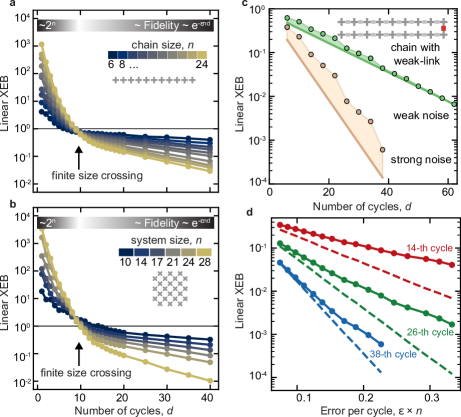
• 약한 연결 모델은 노이즈 주도 전이를 포착하고 XEB가 더 이상 충실도를 충실히 반영하지 않는 경계를 예측한다; 실험은 모델과 일치하는 교차(crossover) 거동을 보인다.
• 1D와 2D 배치에서 XEB 곡선의 교차점이 특정 사이클 수에서 발생하여 동적 위상 전이를 나타낸다; 더 높은 사이클 수는 반분산(anti-concentration)으로 이어지고 그 다음 충실도 주도 XEB가 된다.
• 32 사이클의 67-큐비트 Sycamore 실험은 초-고전 성능과 일치하는 충실도와 난이도를 달성하며, 현실적인 메모리 제약 하에서의 고전 시뮬레이션 비용은 지나치게 큰 것으로 추정된다.
• 수치 및 실험 결과가 함께 임계 노이즈율 εn를 한정하고, 2D 패턴이 시스템 규모에 걸쳐 강건한 약한 노이즈 영역을 제공함을 보인다.

Figure 2: Phase transitions in the Linear Cross-entropy: At low number of cycles, XEB grows with the size of the system. In a noiseless device, XEB will converge to 1 with the number of cycles. In the presence of noise XEB becomes an estimator of the system fidelity. In a and b , we observe experime