[论文解读] Complexity of Supersymmetric Systems and the Cohomology Problem

Chris Cade, P. Marcos Crichigno|arXiv (Cornell University)|Jun 30, 2021

Topological and Geometric Data Analysis参考文献 89被引用 5

一句话总结

该论文确定了超对称系统中上同调问题的量子计算复杂度，证明了 $k$-局部上同调问题为 $\text{QMA}$-完全，并表明估计拟贝蒂数是 $\text{DQC1}$-困难但属于 $\text{BQP}$。此外，研究进一步表明，在结构化系统中，使用超电荷算子 $B$ 而非拉普拉斯算子 $\Delta$ 的变分量子本征求解器（VQE）算法，可将电路深度和测量次数减少 $d+1$ 倍，从而改善算法的缩放性能。

ABSTRACT

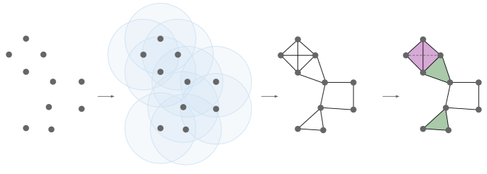
We consider the complexity of the local Hamiltonian problem in the context of fermionic Hamiltonians with $\mathcal N=2 $ supersymmetry and show that the problem remains $\mathsf{QMA}$-complete. Our main motivation for studying this is the well-known fact that the ground state energy of a supersymmetric system is exactly zero if and only if a certain cohomology group is nontrivial. This opens the door to bringing the tools of Hamiltonian complexity to study the computational complexity of a large number of algorithmic problems that arise in homological algebra, including problems in algebraic topology, algebraic geometry, and group theory. We take the first steps in this direction by introducing the $k$-local Cohomology problem and showing that it is $\mathsf{QMA}_1$-hard and, for a large class of instances, is contained in $\mathsf{QMA}$. We then consider the complexity of estimating normalized Betti numbers and show that this problem is hard for the quantum complexity class $\mathsf{DQC}1$, and for a large class of instances is contained in $\mathsf{BQP}$. In light of these results, we argue that it is natural to frame many of these homological problems in terms of finding ground states of supersymmetric fermionic systems. As an illustration of this perspective we discuss in some detail the model of Fendley, Schoutens, and de Boer consisting of hard-core fermions on a graph, whose ground state structure encodes $l$-dimensional holes in the independence complex of the graph. This offers a new perspective on existing quantum algorithms for topological data analysis and suggests new ones.

研究动机与目标

• 确定超对称量子系统中出现的上同调问题的量子复杂度。
• 通过证明超对称基态编码了上同调群，建立哈密顿量复杂度与同调代数之间的桥梁。
• 分析在量子算法中估计贝蒂数和拟贝蒂数的计算复杂度。
• 通过在费米子系统中使用超电荷算子 $B$ 而非拉普拉斯算子 $\Delta$，提升 VQE 的效率。
• 确立 $k$-局部上同调问题属于量子复杂度类 $\text{QMA}$ 的完全性。

提出的方法

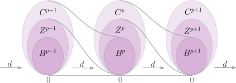
• 使用满足 $d^2 = 0$ 的余边界算子 $d$ 形式化上同调问题，将其映射为具有哈密顿量 $H = \{\mathcal{Q}, \mathcal{Q}^\dagger\}$ 的超对称量子力学系统。
• 利用约旦-维格纳变换将费米子算符映射为量子比特算符，从而实现在量子计算机上的量子模拟。
• 分析超电荷 $B = \mathcal{Q}$ 和拉普拉斯算子 $\Delta = B^2$ 的结构，重点关注其分解为可交换泡利项的形式。
• 提出将 $B$ 和 $\Delta$ 分解为可交换项集合，以减少 VQE 算法中的电路深度和测量次数。
• 证明在独立复形中，使用 $B$ 相较于 $\Delta$ 可将可交换项集合数量减少 $d+1$ 倍，从而改善 VQE 的缩放性能。
• 应用复杂性理论工具，表明拟贝蒂数估计在 $\text{DQC1}$ 下是困难的，但可在 $\text{BQP}$ 中求解。

Figure 3 : Relationship between the cochains $C^{p-1},C^{p},C^{p+1}$ , the cocycles $Z^{p-1},Z^{p},Z^{p+1}$ , and the coboundaries $B^{p-1},B^{p},B^{p+1}$ . The $p$ th cohomology group consists of those elements which are cocycles but not coboundaries, i.e. $H^{p}(d)=Z^{p}/B^{p}$ .

实验结果

研究问题

• RQ1 在超对称系统中，$k$-局部上同调问题的量子计算复杂度是什么？
• RQ2 与使用拉普拉斯算子 $\Delta$ 相比，能否使用超电荷算子 $B$ 来提高 VQE 算法的效率？
• RQ3 作为拓扑数据分析中贝蒂数的代理，估计拟贝蒂数是否在近场量子设备的能力范围内？
• RQ4 底层图的结构如何影响 $B$ 和 $\Delta$ 分解为可交换泡利项的形式？
• RQ5 在费米子格点模型中，超对称基态与上同调群之间存在何种关系？

主要发现

• 证明了 $k$-局部上同调问题为 $\text{QMA}$-完全，确立了其基本的量子难解性。
• 估计拟贝蒂数为 $\text{DQC1}$-困难，表明其对即使纠缠程度较弱的量子计算机也具有难度。
• 拟贝蒂数估计属于 $\text{BQP}$，表明其可在通用量子计算机上高效求解。
• 在独立复形中，使用超电荷 $B$ 而非拉普拉斯算子 $\Delta$ 的 VQE 可将可交换项集合数量减少 $d+1$ 倍，从而改善电路深度和测量次数。
• 约旦-维格纳变换将费米子算符映射为非局域的量子比特算符，但通过结构化图排序可最小化非局域性，从而提升分解效率。
• 本文建立了超对称量子力学与拓扑数据分析之间的直接联系，表明拓扑数据分析中的上同调问题自然地嵌入于量子复杂度类中。

Figure 4 : An example of the TDA pipeline: one starts with a point cloud (left), adds edges between vertices within a certain distance of each other, resulting in a graph $G$ (middle right), from which the clique complex is constructed (right). In this example the complex is connected and has a sing